1 3 4 7 10

Summate Average and Range

Details	Numbers
Enter Your Numbers to Correct With a Comma Betwixt Each E.g: 3, nineteen, ix, seven, 27, 4, eight, xv, 3, 11

Mean, Median, Fashion	Event
Mean (Average):
Median (Heart):
Style (Most Common):

Range & Totals	Results
Range (Biggest - Smallest):
Total Numbers in Gear up:
Ascending Club:
Decending Order:
Fifty-fifty Numbers:
Odd Numbers:

Math Definition

Mean

The average of all the data in a set.

Median

The value in a set which is near close to the centre of a range.

Mode

The value which occures near ofttimes in a data set.

Range

The deviation betwixt the largest and smallest data in a data prepare.

Instance Calculation

Calculate the hateful, median, mode and range for iii, 19, 9, 7, 27, 4, 8, fifteen, 3, 11.

How to Find the Hateful (or Average Value)

To figure the hateful, add up the numbers, 3+3+4+7+viii+9+eleven+15+19+27=106 then divide it by the number of data points 106/10=10.6.

How to Observe the Median

In ascending guild the numbers are three, three, 4, 7, viii, ix, eleven, 15, 19, 27. In that location are ten total numbers, then the 5th and sixth numbers are used to effigy the median. (8+9)/2 = 8.5

If there were 9 numbers in the series rather than ten y'all would take the 5th number and would not demand to boilerplate the ii heart numbers. The 2 middle numbers only need to be averaged when the data set has an fifty-fifty number of information points in information technology.

How to Detect the Mode

The only number which appears multiple times is three, so information technology is the mode.

How to Find the Range

To figure the range subtract the smallest number from the largest number 27-3=24.

Mean, Median and Style: Information Trends, Detecting Anomalies, and Uses in Sports

- Guide Authored by Corin B. Arenas, published on October 17, 2019

In school, we ask the boilerplate score for a test to know if we have a good grade. When information technology comes to buying expensive products, we frequently ask the average price to look for the best deals.

These are but a few examples of how averages are used in real life.

In this section, y'all'll acquire well-nigh the different types of averages and how they're calculated and applied in diverse fields, peculiarly in sports.

What Does the Term 'Average' Mean?

When people describe the 'boilerplate' of a group of numbers, they often refer to the arithmetics mean. This is one out of 3 different types of average, which include median and way.

Types of Boilerplate	Description
Mean	The average of numbers in a grouping.
Median	The middle number in a set up of numbers.
Manner	The number that appears almost often in a prepare of numbers.

In conversational terms, most people just say 'boilerplate' when they're really referring to the mean. Arithmetic mean and average are synonymous words which are used interchangeably, co-ordinate to Dictionary.com.

It's calculated by adding the numbers in a set and dividing it by the total number in the fix—which is what most people do when they're finding the boilerplate. Encounter the example below.

Mean

Set: 8, 12, 9, 7, thirteen, 10
Mean = (8 + 12 + 9 + 7 + 13 + x) / vi
= 59 / 6
= 9.83
The average or arithmetic hateful in this example is ix.83.

Median

The median, on the other hand, is another blazon of average that represents the center number in an ordered sequence of numbers. This works by ordering a sequence of numbers (in ascending order) and so determining the number which occurs at the middle of the set. Meet the instance below.

Boilerplate Median

Set: 22, 26, 29, 33, 39, 40, 42, 47, 53
In this example, 39 is the median or middle value in the fix.

Mode

The fashion is basically the near frequent value that repeats itself in a fix of values. For case, if your set up has 21, 9, fourteen, three, 11, 33, 5, 9, 16, 21, 5, ix, what is the mode?

The respond is ix because this value is repeated 3 times.

In statistics, hateful, median, and mode are all terms used to measure out central tendency in a sample data. This is illustrated by the normal distribution graph below.

The normal distribution graph is used to visualize standard deviation in data assay.  Distribution of statistical data shows how frequent the values in a data set occurs.

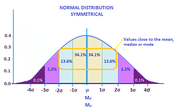
In the graph above, the percentages represent the amount of values that fall within each section. The highlighted percentages basically show how much of the information falls close to middle of the graph.

What is the Relationship Between Mean, Median and Style?

At first glance, it would seem like no connexion exists between mean, median, and style. But there is an empirical relationship that exists in measuring the center of a information ready.

Mathematicians have observed that there is usually a difference between the median and the mode, and information technology is 3 times the difference between the hateful and the median.

The empirical human relationship is expressed in the formula below:
Hateful – Style = iii(Mean – Median)

Let's take the example of population information based on 50 states. For instance, the mean of a population is 7 million, with a median of 4.8 one thousand thousand and way of 1.five million.

• Mean = 7 million
• Median = iv.8 1000000
• Mode = 1.5 1000000

Mean – Way = iii(Hateful – Median)
vii 1000000 – 1.5 million = 3(7 million – 4.viii 1000000)
v.5 million = three(2.2)
5.v million = six.vi 1000000

Take notation: Mathematics professor Courtney Taylor, Ph.D. stated that information technology is not an exact relationship. When you do calculations, the numbers are not always precise. But the corresponding numbers volition be relatively close.

Asymmetrical or Skewed Data

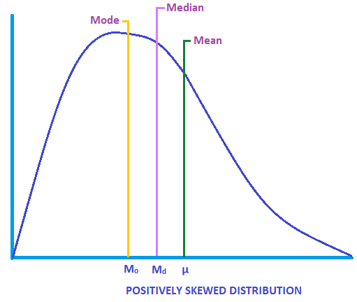
According to Microeconomicsnotes.com, when the values of the mean, median and manner are non equal, the distribution is asymmetrical or skewed. The caste of skewness represents the extent to which a data ready varies from the normal distribution.

When the mean is greater than the median, and the median is greater than the mode (Hateful > Median > Style), it is a positively skewed distribution. It'southward described as 'skewed to the correct' considering the long tail end of the curve is towards the correct.

In the sample graph below, the median and manner are located to the left of the mean.

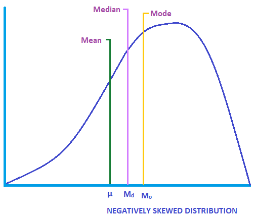
On the other hand, in a negatively skewed distribution, the mean is less than the median, and the median is less than the manner (Hateful < Median < Style). The longtail end is located towards the left side of the graph.

The graph below shows the median and mode located to the correct side of the hateful.

Varying Mean from Median: Resistant Numerical Summaries

In a data set, when the mean is high, a reader might assume the median volition also be high. However, this does not e'er follow.

The difference betwixt mean and median becomes apparent when a information gear up has an outlying disparate value. This situation calls attention to the concept of resistant numerical summaries. A resistant statistic is a numerical summary wherein extreme numbers do not take a substantial affect on its value.

Permit'southward show this by demonstrating how Bill Gates' presence impacts mean and median wealth when he walks into a room.

For case, 10 people are having dinner at a restaurant. Let's call it set A. The table below shows their income from everyman to highest.

Name	Annual Income
Raffy	$33,000
Jessie	$38,000
Corin	$39,000
Paul	$42,000
Kat	$46,000
Luigi	$49,000
Carl	$52,000
Susan	$sixty,000
Miguel	$68,000
John	$79,000

The total income of the people in the restaurant is $506,000, with a mean income of $50,600.

Since there are 10 people in the set, to get the median, we have to add together the v^thursday and 6^thursday values (Kat and Luigi'southward annual income) and divide it by ii.

Median = (46,000 + 49,000) / 2= 95,000/ii
= 47,500
The median income of the grouping is $47,500.

The range is the deviation between the everyman income (Raffy) and the highest income (John), which is $46,000.

Ready A Annual Income

Total Income	$506,000
Mean	$506,000
Median	$47,500
Range	$46,000

Now, if John leaves the eatery and Beak Gates walks in, how will it affect the group'south almanac income stats? Let'southward telephone call this next group set B.

According to Forbes, Bill Gates made $90 billion from 2017 to 2018.

Name	Annual Income
Raffy	$33,000
Jessie	$38,000
Corin	$39,000
Paul	$42,000
Kat	$46,000
Luigi	$49,000
Carl	$52,000
Susan	$60,000
Miguel	$68,000
Bill Gates	$90,000,000,000

Set B Annual Income

Total Income	$90,000,427,000
Mean	$9,000,042,700
Median	$47,500
Range	$89,999,967,000

With Bill Gates, the total income is now $xc billion plus the lower income of the people in the restaurant. The mean income and the range of the grouping is at present too loftier.

 Still, the median remains the same at around $47,500.

The median shows it's a meliorate indication of people'south actual financial status. Besides, we can say Bill Gates is an outlier with an annual income that hits billions.

This example shows that the mean and range are not resistant to extreme values. While the median, as a numerical summary, generally exhibits resistance.

What does this tell us? The presence of extreme values or outliers bespeak that a distribution is skewed. Extreme values typically pull the mean toward the direction of the tail.

The Significance of Identifying Skewness

Observing skewness in a graph gives analysts a clearer thought of a information set's tendency. For instance, if you collected data from 500 students that took the Scholastic Assessment Exam, you'd want to know the score trend.

If you plot the data in a graph, yous'd know it'southward positively skewed if there are few high scores and most of the values are amassed towards the lower side of the scale. If the scores tend toward the higher side of the calibration, with few depression scores, the distribution is negatively skewed.

In finance, investors take note of skewness when they analyze return distribution. This is of import because information technology allows them to see the farthermost ranges of the data instead of just focusing on the average values.

A distribution shows skewness (degree of disproportion) or kurtosis when the returns fall outside the normal distribution. Kurtosis measures the outliers in either tail of a skewed graph. Information technology calculates the degree to which a graph is peaked compared to a normal distribution.

How does it help investors? Observing skewness or kurtosis helps analysts predict risks that that effect when a model following normal distribution is compared to a information gear up with a tendency for higher standard deviation. The risk is determined by calculating how far the numbers are from the normal distribution.

How to Identify Information Anomalies

In statistics, outliers or anomalies are unusual observations that do non belong to a certain population.

When placed in a graph, these are points that fall far away from the data set up's values. Researchers normally find outliers based on big, well-structured data.

How dissimilar should a value be to be considered an outlier? To decide this, you can employ the interquartile range (IQR).

IQR is described as a 5 number summary, which contains:

• The minimum value of a data set
• The first quartile (Q₁) – Which is a quarter of the style through the sequence of a information ready
• The median
• The third quartile (Q_three) Which is 3 quarters of the way through the sequence of all information
• The maximum value of the data set

The interquartile range (IQR) is also similar to range but is considered a less sensitive to extreme values (resistant statistic). To discover information technology, y'all must take the first quartile and subtract the 3rd quartile. This shows how data is spread around the median.

IQR = Q₃ – Q₁

Detecting Outliers Using IQR

Practically all sets of data can be described by the 5 number summary. Here'southward how you tin utilise IQR to find outliers:

1. Compute the interquartile range for the information set
2. Multiply the IQR by i.v
3. Add IQR ten one.5 to the third quartile. The dominion: Whatever value greater that this is an outlier.
4. Decrease IQR x 1.five from the kickoff quartile. The rule: Any value less than this is an outlier.

Here's an example. Suppose y'all're finding the outlier for the data fix beneath:
1, 5, 6, 6, ix, x,  10, eleven, 12, 13, 18
5 number summary:

• Minimum value = ane
• Q_ane = vi
• Median = 10
• Q_iii = 12
• Maximum value = eighteen

IQR = Q_iii – Q₁
= 12 – 6
IQR = 6

IQR x 1.5 = ?
6 x one.5 = nine
ix + Q₃ = ?
9 + 12 = 21 (any value greater than 21 is an outlier)

6 – Q₁ = ?
6 – nine = -3 (any value less that -3 is an outlier)

So far, no value is less than -three or greater than 21 in the ready. Though the maximum value 18 is 5 points more than xiii, it is not considered an outlier for this data set.

How Statistic Averages are Used in Sports Analytics

In sports analytics, researchers assemble statistics to measure the potential and ability of professional athletes.

According to Competitive Edge Athletic Performance Heart, sports functioning metrics are relevant to overall athletic development. To attain success in any sports field, individuals must reach sure levels of athleticism to compete at advanced levels.

In fact, many professional sports teams consult statisticians to help athletes track their competitive reward. This guides them in improving their force and conditioning routines.

Tracking performance metrics helps athletes practice 4 crucial things:

1. Helps them know their current level or baseline.
2. One time they amend, information technology allows them to compete at college sports levels.
3. Allows athletes to identify private preparation needs.
4. Can help lower the risk of injuries.

Popular Sports Averages

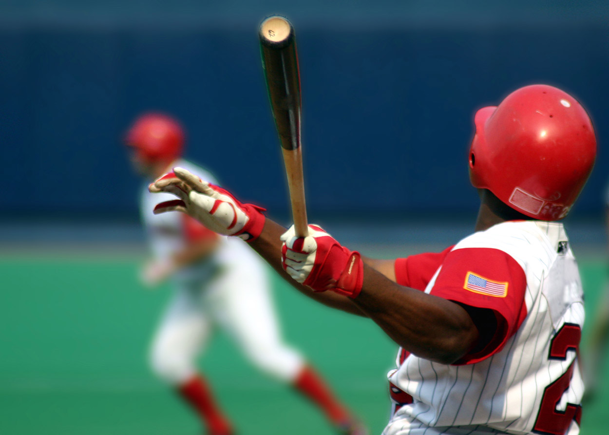
Batting average (BA) is a functioning statistic used in baseball, cricket and softball. It measures the number of average runs a player can score before getting out.

It's the oldest measuring tool that gauges a batter's success. College BA ways the batter has greater potential to score runs without getting an out.

The BA is calculated by dividing a player's hits by his total at-bats, for a value between .000 and 1.000.

According to the Major League Baseball website, the league-broad BA in recent years has remained around .260. For the game's best batters, they can exceed .300.

Nonetheless, some exceptional athletes accept hitting higher up .400, which is 4 hits for every 10 at-bats. MLB states no player has washed this throughout a total flavour since Ted Williams (.406) of Boston Red Sox in 1941.

In the strike-shortened 1994 season Tony Gwynn came close to hitting 400, batting 394 with 164 hits on 419 at bats in 110 games.

Here'due south a table of MLB players showing the regular season batting boilerplate leaders from 1985 to 2019 :

Year	National League Leader	NL Team	BA	American League Leader	AL Squad	BA
2019	Christian Yelich	MIL	.329	Tim Anderson	CHW	.335
2018	Christian Yelich	MIL	.326	Mookie Betts	BOS	.346
2017	Charlie Blackmon	COL	.331	Jose Altuve	HOU	.346
2016	DJ LeMahieu	COL	.348	Jose Altuve	HOU	.338
2015	Dee Gordon	MIA	.333	Miguel Cabrera	DET	.338
2014	Justin Morneau	COL	.319	Jose Altuve	HOU	.341
2013	Michael Cuddyer	COL	.331	Miguel Cabrera	DET	.348
2012	Buster Posey	SFG	.336	Miguel Cabrera	DET	.330
2011	Jose Reyes	NYM	.337	Miguel Cabrera	DET	.344
2010	Carlos Gonzalez	COL	.336	Josh Hamilton	TEX	.359
2009	Hanley Ramirez	FLA	.342	Joe Mauer	MIN	.365
2008	Chipper Jones	ATL	.364	Joe Mauer	MIN	.328
2007	Matt Holliday	COL	.340	Magglio Ordonez	DET	.363
2006	Freddy Sanchez	PIT	.344	Joe Mauer	MIN	.347
2005	Derrek Lee	CHC	.335	Michael Young	TEX	.331
2004	Barry Bonds	SFG	.362	Ichiro Suzuki	Sea	.372
2003	Albert Pujols	STL	.359	Beak Mueller	BOS	.326
2002	Barry Bonds	SFG	.370	Manny Ramirez	BOS	.349
2001	Larry Walker	COL	.350	Ichiro Suzuki	SEA	.350
2000	Todd Helton	COL	.372	Nomar Garciaparra	BOS	.372
1999	Larry Walker	COL	.379	Nomar Garciaparra	BOS	.357
1998	Larry Walker	COL	.363	Bernie Williams	NYY	.339
1997	Tony Gwynn	SDP	.372	Frank Thomas	CHW	.347
1996	Tony Gwynn	SDP	.353	Alex Rodriguez	SEA	.358
1995	Tony Gwynn	SDP	.368	Edgar Martinez	Ocean	.356
1994	Tony Gwynn	SDP	.394	Paul O'Neill	NYY	.359
1993	Andres Galarraga	COL	.370	John Olerud	TOR	.363
1992	Gary Sheffield	SDP	.330	Edgar Martinez	SEA	.343
1991	Terry Pendleton	ATL	.319	Julio Franco	TEX	.341
1990	Willie McGee	STL	.335	George Brett	KCR	.329
1989	Tony Gwynn	SDP	.336	Kirby Puckett	MIN	.339
1988	Tony Gwynn	SDP	.313	Wade Boggs	BOS	.366
1987	Tony Gwynn	SDP	.370	Wade Boggs	BOS	.363
1986	Tim Raines	Monday	.334	Wade Boggs	BOS	.357
1985	Willie McGee	STL	.353	Wade Boggs	BOS	.368

In basketball game, field goal percentage (FG) is used to measure how effectively a team scores a ball during a game.

FG considers all shots taken past a player. However, it doesn't include gratis throws that are measured independently equally complimentary throw pct.

The formula for FG is the number of successful shots divided by the full number of shot attempts.

An FG of .500 or 50% and upwardly is usually considered a skilful pct. According to Basketball Reference, the active histrion with the highest percentage is currently DeAndre Hashemite kingdom of jordan, with 66.96%.

Notable basketball game players like Michael Hashemite kingdom of jordan take an FG of 49.69% with a ranking of 151, while Lebron James ranks at 111 with 50.42%. Hall of famers like Kareem Abdul-Jabbar ranks at 14 with 55.95%, while Magic Johnson ranks at 64 with 51.97%.

Basketball game Reference identified the 4 factors that help teams win games:

• Shooting (xl%)
• Turnovers (25%)
• Rebounding (20%)
• Free Throws (15%)

Out of the 4, shooting is the most important factor, followed by turnovers, rebounding and free throws. However, others would argue that apart an effective field goal percentage, a game is won with a solid defence strategy.

Below is a table of NBA players with the highest field goal percentage.

Active players are in assuming.
* Indicates a member of the Hall of Fame

Rank	Name	FG%
1.	DeAndre Jordan	.6696
2.	Artis Gilmore*	.5990
3.	Tyson Chandler	.5960
four.	Dwight Howard	.5828
v.	Shaquille O'Neal*	.5823
half-dozen.	Marking W	.5803
7.	Steve Johnson	.5722
viii.	Darryl Dawkins	.5720
9.	James Donaldson	.5706
10.	JaVale McGee	.5697
	Amir Johnson	.5697
12.	Bo Outlaw	.5673
13.	Jeff Ruland	.5637
14.	Kareem Abdul-Jabbar*	.5595
xv.	Jonas Valančiūnas	.5583
16.	Kevin McHale*	.5538
17.	Marcin Gortat	.5514
18.	Bobby Jones*	.5504
xix.	Cadet Williams	.5492
xx.	Nenê Hilário	.5478

Many field goal percentage leaders are big men who tend to dunk & shoot other high percentage inside shots. In recent years the three-point shot has become more widely used. A mark of a groovy all around shooting functioning is 50-40-90, where a player has a fifty% FG, forty% from 3-point range, and 90% from the costless throw line.

The Bottom Line

There are three types of averages, and these are the mean, median and manner. Out of the three, the most commonly used is the arithmetics mean. It'south determined by adding all the values in a ready and dividing it by the full number of factors.

Calculating mean, median and mode allows researchers to observe normal distribution or skewness in a graph. In finance, investors use this to measure the gamble of return distribution. To detect statistical outliers, analysts apply the interquartile range.

Calculating averages is peculiarly relevant in sports analytics. It's used to set benchmarks and improve able-bodied performance. Metrics help athletes streamline forcefulness and conditioning routines, as well as avoid injuries.

About the Author

Corin is an agog researcher and writer of financial topics—studying economic trends, how they affect populations, as well every bit how to assistance consumers make wiser financial decisions. Her other characteristic articles can exist read on Inquirer.cyberspace and Manileno.com. She holds a Master'southward degree in Artistic Writing from the Academy of the Philippines, i of the top bookish institutions in the world, and a Bachelor's in Advice Arts from Miriam College.

When in Doubt, Autosum ;)

1 3 4 7 10,

Source: https://www.calculators.org/math/mean-median-mode.php

Posted by: propsttwithe88.blogspot.com

Share this post